Mencoba TTS Bahasa Indonesia dengan VITs dan Meta MMS

Sudah lama saya ingin mencoba (membuat) teknologi text-to-speech (TTS) atau speech synthesis bahasa Indonesia. Percobaan pertama saya beberapa tahun lalu gagal. Disini reponya: Expressive-FastSpeech2. Pada percobaan tersebut, saya langsung mencoba membuat suara (bukan Bahasa Indonesia) yang memiliki emosi, seperti suara orang marah, sedih, atau senang. Alih-alih suara, saya hanya mendengar derau/bising saja dari algoritma FastSpeech2.

Ketika Meta/Facebook mengumumkan salah satu riset mereka, yakni MMS (Massively Multilingual Speech), saya langsung tertarik mencobanya. MMS bisa diaplikasikan untuk ASR (automatic speech recognition, atau STT, speech-to-text) dan TTS. Untuk TTS, sepemahaman saya, Meta hanya mengaplikasikan dataset yang besar pada Variational Inference with adversarial learning for end-to-end Text-to-Speech (VITS). Saya coba ASRnya tidak lebih baik dari OpenAI Whisper, khususnya dari sisi latency. Saya coba TTSnya, kebetulan hasilnya memuaskan, khususnya untuk yang belum pernah berhasil membuat TTS sendiri.

Repository

Untuk keperluan TTS ini, saya buat repository khusus di Github: TTS-Bahasa. TTS-Bahasa sebenarnya tidak khusus untuk bahasa Indonesia, tapi semua bahasa yang didukung oleh MMS (ada lebih dari 1000 bahasa). Repo tersebut saya adaptasi dari tutorial di laman MMS, yakni tutorial Google Colabnya. Saya hanya menambahkan satu skrip python CLI (command line interface) untuk memudahkan pembuatan audio file suara sintesis berdasarkan input kalimat. Contohnya seperti ini.

python3 mms_tts_ind.py --text "Selamat datang di Indonesia"

Suara berbahasa Indonesia akan diperdengarkan setelah eksekusi program selesai (berbunyi: "Selamat datang di Indonesia"). Luaran suara tersebut juga bisa disimpan dalam format WAV atau MP3, misalnya.

python3 mms_tts_ind.py --text "Selamat datang di Indonesia" -s -o selamat_datang.wav 

Untuk mencobanya, tidak perlu menginstall. Cukup clone repo tersebut, dan ikuti petunjuk di READMEnya. Jika ada kendala, anda bisa membuka "issues" di repo tersebut.

Demo

Jika anda bukan programmer, coder, researcher, mahasiswa teknik, atau tidak terbiasa dengan Python, anda bisa langsung mencoba demo-nya disini: https://bagustris.github.io/tts-bahasa/.

Acoustic Feature Extraction with Transformers

The example in Transformers' documentation here shows how to use the wav2vec 2.0 model for automatic speech recognition. However, there are two crucial issues in that example. First, we usually use our data (set) instead of their (available) dataset. Second, we need to extract acoustic features (the last hidden states instead of logits). The following is my example of adapting Transformers to extract acoustic embedding given any audio file (WAVE) using several models. It includes the pooling average from frame-based processing to utterance-based processing for given any audio file. You don't need to perform the pooling average if you want to process your audio file in frame-based processing (remove the `.mean(axis=0)` in the variable `last_hidden_states`).

Basic syntax: wav2vec2 base model

This is the example from the documentation. I replaced the use of the dataset with the defined path of the audio file ('00001.wav').

from transformers import Wav2Vec2Processor, Wav2Vec2Model
import torchaudio
import torch
# load model
processor = Wav2Vec2Processor.from_pretrained("facebook/wav2vec2-base-960h")
model = Wav2Vec2Model.from_pretrained("facebook/wav2vec2-base-960h")

# audio file is decoded on the fly
array, fs = torchaudio.load("/data/A-VB/audio/wav/00001.wav")
input = processor(array.squeeze(), sampling_rate=fs, return_tensors="pt")

# apply the model to the input array from wav
with torch.no_grad():
    outputs = model(**input)

# extract last hidden state, compute average, convert to numpy
last_hidden_states = outputs.last_hidden_state.squeeze().mean(axis=0).numpy()

# print shape
print(f"Hidden state shape: {last_hidden_states.shape}")
# Hidden state shape: (768,)

The syntax for the wav2vec2 large and robust model

In this second example, I replace the base model with the large and robust model without finetuning. This example is adapted from here. Note that I replaced 'Wav2Vec2ForCTC' with 'wav2vec2Model'. The former is used when we want to obtain the logits (for speech-to-text transcription) instead of obtaining the hidden states.

from transformers import Wav2Vec2Processor, Wav2Vec2Model
import torch
import torchaudio

# load model
processor = Wav2Vec2Processor.from_pretrained(
    "facebook/wav2vec2-large-robust-ft-swbd-300h")
model = Wav2Vec2Model.from_pretrained(
    "facebook/wav2vec2-large-robust-ft-swbd-300h")

# audio file is decoded on the fly
array, fs = torchaudio.load("/data/A-VB/audio/wav/00001.wav")
input = processor(array.squeeze(), sampling_rate=fs, return_tensors="pt")

with torch.no_grad():
    outputs = model(**input)

last_hidden_states = outputs.last_hidden_state.squeeze().mean(axis=0).numpy()
# printh shape
print(f"Hidden state shape: {last_hidden_states.shape}")

You can replace "facebook/wav2vec2-large-robust-ft-swbd-300h" with "facebook/wav2vec2-large-robust-ft-libri-960h" for the larger fine-tuned model.

 For other models, you may need to change `Wav2Vec2Processor` with `Wav2Vec2FeatureExtractor` for processor variable. In my case, this is needed for the following models:

• facebook/wav2vec2-large-robust
• facebook/wav2vec2-large-xlsr-53

The syntax for the custom model (wav2vec-R-emo-vad)

The last one is the example of the custom model. The model is wav2vec 2.0 fine-tuned on the MSP-Podcast dataset for speech emotion recognition. This last example differs from the previous one since the configuration is given by the authors of the model (read the code thoroughly to inspect the details). I replaced the dummy audio file with the real audio file. It is assumed to process in batch (with batch_size=2) by replicating the same audio file.

import torch
import torch.nn as nn
from transformers import Wav2Vec2Processor
from transformers.models.wav2vec2.modeling_wav2vec2 import (
    Wav2Vec2Model,
    Wav2Vec2PreTrainedModel,
)
import torchaudio


class RegressionHead(nn.Module):
    r"""Classification head."""

    def __init__(self, config):

        super().__init__()

        self.dense = nn.Linear(config.hidden_size, config.hidden_size)
        self.dropout = nn.Dropout(config.final_dropout)
        self.out_proj = nn.Linear(config.hidden_size, config.num_labels)

    def forward(self, features, **kwargs):

        x = features
        x = self.dropout(x)
        x = self.dense(x)
        x = torch.tanh(x)
        x = self.dropout(x)
        x = self.out_proj(x)

        return x


class EmotionModel(Wav2Vec2PreTrainedModel):
    r"""Speech emotion classifier."""

    def __init__(self, config):

        super().__init__(config)

        self.config = config
        self.wav2vec2 = Wav2Vec2Model(config)
        self.classifier = RegressionHead(config)
        self.init_weights()

    def forward(
            self,
            input_values,
    ):

        outputs = self.wav2vec2(input_values)
        hidden_states = outputs[0]
        hidden_states = torch.mean(hidden_states, dim=1)
        logits = self.classifier(hidden_states)

        return hidden_states, logits


def process_func(
    wavs,
    sampling_rate: int
    # embeddings: bool = False,
):
    r"""Predict emotions or extract embeddings from raw audio signal."""

    # run through processor to normalize signal
    # always returns a batch, so we just get the first entry
    # then we put it on the device
    # wavs = pad_sequence(wavs, batch_first=True)
    # load model from hub
    device = 'cpu'
    model_name = 'audeering/wav2vec2-large-robust-12-ft-emotion-msp-dim'
    processor = Wav2Vec2Processor.from_pretrained(model_name)
    model = EmotionModel.from_pretrained(model_name)

    y = processor([wav.cpu().numpy() for wav in wavs],          
                   sampling_rate=sampling_rate,
                   return_tensors="pt",
                   padding="longest"
        )
    y = y['input_values']
    y = y.to(device)


    y = model(y)

    return {
        'hidden_states': y[0],
        'logits': y[1],
    }


## test to an audiofile
sampling_rate = 16000
signal = [torchaudio.load('train_001.wav')[0].squeeze().to('cpu') for _ in range(2)]

# extract hidden states
with torch.no_grad():
    hs = process_func(signal, sampling_rate)['hidden_states']
print(f"Hidden states shape={hs.shape}")

Please note for all models, the audio file must be sampled with 16000 Hz, otherwise, you must resample it before extracting acoustic embedding using the methods above. It may not throw an error even if the sampling rate is not 16000 Hz but the results, hence, is not valid since all models were generated based on 16 kHz of sampling rate speech datasets. 

You may also want to extract acoustic features using the opensmile toolkit. The tutorial for Windows users using WSL is available here: http://bagustris.blogspot.com/2021/08/extracting-emobase-feature-using-python.html.

Happy reading. Don't wait for more time to apply these methods to your own audio file.

Extracting Emobase Feature Using Python-Opensmile under Windows (WSL)

This article documents my steps to extract acoustic features with "emobase" configuration on opensmile-python under Windows. I used WSL (Window Sub-System for Linux) with Ubuntu Latest (20.04). Click each image for larger size and clarity.

0. Windows Version

Here is my Windows version in which I experimented with. Other versions may give errors. To show your version, simply press the Windows button and type "about PC".

Edition	        Windows 10 Pro
Version	        20H2
Installed on	‎4/‎2/‎2021
OS build        19042.1083
Experience      Windows Feature Experience Pack 120.2212.3530.0

1. Activate WSL2

Here are the steps to activate WSL2 on Windows 10. WSL2 only works on Windows 10 version 1903 or higher, with Build 18362 or higher. For the older version, you can use WSL instead of WSL2.
a. Activate WSL using PowerShell. Press the Windows key, and enter the following.

 dism.exe /online /enable-feature /featurename:Microsoft-Windows-Subsystem-Linux /all /norestart 

b. Install Linux kernel update package. Download from here.
https://wslstorestorage.blob.core.windows.net/wslblob/wsl_update_x64.msi
Double click and install that .msi package.
Select WSL2 as default.

 wsl --set-default-version 2 

You need to ensure the wsl version after installing Ubuntu distro below.

2. Install Ubuntu

Press windows key and type "Microsoft Store". I choose Ubuntu (latest) instead of Ubuntu 20.04 or other versions. See image below; I already installed it.

Ensure that Ubuntu uses WSL2 as default. Check-in PowerShell with the following command (wsl -l -v).

Then click launch Ubuntu from the previous image/step, or you can type "Ubuntu" di search dash.
When launching Ubuntu for the first time, you will be prompted for the user name and password. Remember this credential. See the image below for example.

3. Install Python and pip

In Ubuntu do/type

 sudo apt update && sudo apt -y upgrade 

Enter your password. Type "y" when it is prompted.
Install Python using apt. I chose python3.7 as follows.

 sudo apt install python3.7-full 

Type "y" when it asked. See the image below for reference.

Test if the installation is successful. Type "python3.7" in Ubuntu to enter python3.7 console.

Next, we need pip to install python packages. Hence, we need to install pip first as follows.

 python3.7 -m ensurepip --upgrade 

4. Install Python-Opensmile

Since this version of python in Ubuntu is already equipped with pip, we can directly use it to install opensmile.

 python3.7 -m pip install opensmile 

See the image below for a reference.

Same as previous step, I installed IPython for my convenience. You may also need to install numpy, scipy, and matplotlib.

 python3.7 -m pip install ipython numpy scipy audb

We also need to install sox since it is required by opensmile

 sudo apt install sox 

5. Extract Emobase Feature

Now is the time to use opensmile. First, open IPython console for this python3.7.

 python3.7 -m IPython 

Import Opensmile and download emodb dataset with a specific configuration.
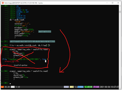
See the image below for your reference. Skip the parts with red cross since they contain errors (I forgot to add a comma between arguments).

Configure opensmile to extract EMOBASE feature.

smile = opensmile.Smile(
    feature_set=opensmile.FeatureSet.emobase,
    feature_level=opensmile.FeatureLevel.Functionals,
)
smile.feature_names

See image below for your reference. You can change feature_level value to "opensmile.FeatureLevel.LowLevelDescriptors" if you want LLD (LowLevelDescriptors, extracted per frame) instead of functionals (statistics of LLD). The number of emobase functional is 988 features [len(smile.features_names)].

Finally, we extract acoustic features based on these configuration.

smile.process_signal(
    signal,
    sampling_rate
)

See below image for your reference.

That's all. Usually, I save the extracted acoustic features in other format like numpy .npy files or .csv files. From my experience, this is my first extraction of emobase feature set. Previously I used gemaps, egemaps, compare2016, and emo_large configuration. Let see if this kind of feature set has advantages over others. Although intended for Windows 10, this configuration may also works for other distribution. Still, I prefer to use Ubuntu since the process is simple and straightforward. No need to set WSL2 and other things just pip and pip.

The full script to extract emobase functional features from all utterances in emodb dataset is given below. Please note that it takes a long time to process since it will download all utterances in emodb dataset according to "audb" format and extract acoustic features from them.

Example 1: Extract emobase feature from an excerpt of emodb dataset and save it as an .npy file.

import os
import time

import numpy as np
import pandas as pd

import audb
import audiofile
import opensmile

sr = 16000

# if you change code below, it will download the dataset again 
db = audb.load(
    'emodb',
    version='1.1.1',
    format='wav',
    mixdown=True,
    sampling_rate=sr,
    full_path=False,
    verbose=True,
)

smile = opensmile.Smile(
    feature_set=opensmile.FeatureSet.emobase,
    feature_level=opensmile.FeatureLevel.Functionals,
)

# If you run this program for the second time
# comment the whole db above and change db.root and db.files to (uncomment)
# db_root = audb.cached().index[0]
# db_files = pd.read_csv('/home/bagus/audb/emodb/1.1.1/fe182b91/db.files.csv')['file']

feats = []
for i in db.files:
    file = os.path.join(db.root, db.files[i])
    signal, _ = audiofile.read(
            file,
            always_2d=True,
            )
    feat = smile.process_signal(
            signal,
            sr
            )
    feats.append(feat.to_numpy().reshape(-1))

# this will save all emodb emobase feature in a single npy file
# make sure you have 'data' dir first
np.save('data/emodb_emobase.npy', feats)
  

Example 2: Extract emobase features from files under a directory ("ang") and save it in a csv file.

import os
import opensmile
import numpy as np
import glob
#from scipy.io import wavfile

# jtes angry path, 50 files
data_path ="/data/jtes_v1.1/wav/f01/ang/"
files = glob.glob(os.path.join(data_path, "*.wav"))
files.sort()

# initiate opensmile with emobase feature set
smile = opensmile.Smile(
    feature_set=opensmile.FeatureSet.emobase,
    feature_level=opensmile.FeatureLevel.Functionals,
)
smile.feature_names

# read wav files and extract emobase features on that file
feat = []

for file in files:
    print("processing file ... ", file)
    #sr, data = wavfile.read(file)
    #feat_i = smile.process_signal(data, sr)
    feat_i = smile.process_file(file)
    feat.append(feat_i.to_numpy().flatten())

# save feature as a csv file, per line, with comma
np.savetxt("jtes_f01_ang.csv", feat, delimiter=",")

  

If you face problems during following this article, let me see in comments below.

Reference:
[1] https://docs.microsoft.com/en-us/windows/wsl/install-win10
[2] https://audeering.github.io/opensmile-python/usage.html

Data yang besar mengalahkan algoritma yang baik

Dalam sebuah workshop yang saya ikuti setahun dua tahun yang lalu di Trieste, seorang pemateri dengan pedenya menyampaikan: "bigger data win over good algorithm", data yang besar mengalahkan algortima yang baik. Saya tercengang. Benarkah...? Selama sekolah, S1~S2, saya diajari dan dituntut untuk menghasilkan algoritma yang baik dari data pengukuran fisis untuk aplikasi kontrol, prediksi, diagnosa dan lain sebagainya. Namun sekarang paradigmanya berubah, bukan bagaimana meng-improve algoritma, tapi mempebesar jumlah data. Tidak sepenuhnya benar memang, namun ini jauh lebih mudah. Akan lebih mudah mengakuisisi lebih banyak data daripada mengimprove/memodifikasi algoritma yang biasanya membutuhkan matematika yang cukup rumit.

Benar adanya, tak semata-mata algoritma/metode yang baik, tapi juga data yang banyak. Gampangannya, orang yang yamg "pintar" tapi jarang belajar dibanding dengan orang yang "rajin" belajar dari banyak data. Pengalaman menunjukkan, tipe orang disebut terakhir lebih banyak berhasilnya daripada tipe orang yang disebut pertama.

Analogi lagi, data vs algoritma: mana yang lebih penting adalah seperti membandingkan mana yang lebih dulu: telur atau ayam. Awalnya saya, mungkin seperti kebanyakan orang juga, berpikiran telur lebih dahulu. Alasannya: telur lebih rigid, lebih statis, dan lebih kecil daripada ayam. Namun hasil penelitian membuktikan bahwa ayam lebih dahulu daripada telur (artinya Tuhan menciptakan ayam dulu, ini lebih masuk akal). Begitu juga dengan data vs algoritma: data-lah akhirnya yang menang, tentunya data yang banyak, big atau bahkan very big.

Jadi tunggu apa lagi? Cari data sebanyak-banyaknya, seakurat mungkin! Mengumpulkan data tidak sesulit membangun algortima. Kalau membangun algortima, kita butuh mikir exktra, menurunkan rumus matematik, dan mengimplementasikannya dalam bahasa pemrograman. Sedangkan untuk mengumpulkan data, kita cuma butuh waktu, keuletan, dan ketekunan. Contohnya untuk data teks, kita perlu sabar dan rajin mengumpulkan kalimat, tokenisasi, mengetik dan sebagaiknya. Untuk data suara, kita perlu merekam, mengedit dan memanipulasi (tambahkan noise, hilangkana noise, dsb). Jauh lebih mudah untuk memperbanyak data daripada memperbaiki algoritma.

Garbage In Garbage Out
Salah satu prinsip yang penting dalam machine learning dan pengenalan pola adalah "data yang baik", berkualitas. Jika data yang kita masukkan adalah sampah, maka hasilnya juga sampah. Maka, selain memperbanyak data, yang harus kita perhatikan adalah kualitas data tersebut. Jangan sampai data yang kita latih, misal dengan deep learning, merupakan data sampah, sehingga hasilnya juga sampah. Disinilah pentingnya preprocessing.

Berapa data yang "besar" itu?

Pertanyaanya selanjutnya, jika data yang besar mengalahkan algoritma yang baik, seberapa besar data yang besar itu? Ian Goodfellow et al. dalam bukunya "Deep learning" berargumen sebagai berikut,

As of 2016, a rough rule of thumb is that a supervised deep learning algorithm will generally achieve acceptable performance with around 5,000 labeled examples per category, and will match or exceed human performance when trained with a dataset containing at least 10 million labeled examples. Working successfully with datasets smaller than this is an important research area, focusing in particular on how we can take advantage of large quantities of unlabeled examples, with unsupervised or semi-supervised learning.

 Jadi, 5000 data yang terlabeli dengan benar merupakan data minimal dari sisi best practice. Tenju saja, semakin besar semakin baik.

Referensi:

1. Alon Halevy, P. Norvig, F. Pereira, "The Unreasonable Effectiveness of Data". Available online:https://static.googleusercontent.com/media/research.google.com/ja//pubs/archive/35179.pdf
2. https://www.datasciencecentral.com/profiles/blogs/data-or-algorithms-which-is-more-important

Modeling Acoustic Mixture in Semi Anechoic Room

How-to: Measure Impulse Response with Aliki

Aliki is software to measure room impulse response. It's free and open source. On a dynamic system, impulse response is its output(response) when presented with a brief input signal (impulse). For room acoustic, impulse response can be used to measure acoustic characteristics like reverberation time, early decay time, later decay time and speech intelligibility.

How to measure room impulse response? Here is how, with a software called Aliki (free and open source).

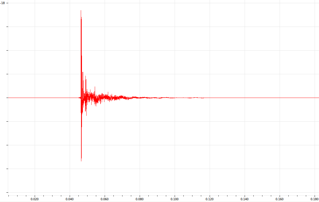
Impulse response of semi-anechoic room in VibrasticLab

Installation

In Ubuntu, it is easy to install Aliki using apt-get:

sudo apt-get install aliki

It will install Aliki (gui) and its dependencies.

Step-by-step :

Wavplot and Wavplay

Matlab has their built in function to play .wav file, but it didn't work in Unix and Linux-based OS, because the wavplay function only supported in Windows. Moreover, I want to plot waveform of .wav file in single command, so I don't need to wavread it before plot. For those two purposes, I made two shorts function namely wavplot and wavfile.

Wavplot
wavplot is simple function to plot .wav file. Why I need it? because I continuously working with .wav file, and I want to plot it directly to get information of sound file via its waveform. Here the code of wavplot function.

function wavplot(wavFile)
% wavplot(wavFile) plot waveform and spectrum of wav file
% bagus@ep.its.ac.id

if nargin>1
    fprintf('Usage: wavplot(wavFile \n');
    return;
end;

[y, fs]=wavread(wavFile);
plot(y)
end

How to use it? it is simple. If you have .wav file, for example it has name tone.wav and you are in the current directory of Matlab command window, you can directly plot it with this function,

wavplot('tone.wav')

And it will plot the wav file like the following,

Output of wavplot function

Deteksi Multi Pitch Berdasarkan Jumlahan Harmonik

Pitch merupakan persepsi telinga manusia atas frekuensi dasar (suara). Deteksi maupun estimasi pitch banyak dipelajari dan digunakan untuk beberapa aplikasi seperti pemisahan suara, pengenalan suara atau untuk tuning alat musik.

Output progam

Berdasarkan paper Ansi Klapuri pada tahun 2006, estimasi multi-pitch ini dapat didekati dengan jumlahan harmonik. Pendekatan ini secara konseptual "sangat simpel" dan efisien secara komputasi. Ide dasarnya adalah dengan menghitung saliance, strength atau power dari kandidat F0 sebagai jumlah bobot amplitudo harmonik-harmoniknya. Pemetaan dari spektrum Fourrier menjadi "F0 salience spectrum"  didapatkan dari optimisasi data training.

Saliance dapat dihitung dari jumlah bobot amplutido dari harmonik sebagai berikut,

dimana f adalah frekuensi harmonik ke-n, dan g adalah bobot parsial harmonik m dari periode tau.

Metode

Menghitung MSE dari .wav file di Matlab

MSE (mean squared error) adalah salah satu standar evaluasi obyektif (objective evaluation) pada dunia sains dan teknik, baik pada cabang ilmu fisika, kimia, biologi, informatika, elektronika dan bidang rekayasa yang lain. Misalkan kita mempunyai sebuah data atau sinyal (suara, gambar, dll) yang telah kita manipulasi (enhancement, separation, improvement) dan kita ingin membandingkan sinyal output (estimasi, enhanced, separated) dengan sinyal aslinya, maka kita membandingkan sinyal asli dan sinyal estimasi tersebut dengan teknik MSE dengan salah satu syarat: panjang sinyalnya sama.

Secara matematik, MSE dirumuskan sebagai berikut,

Sedangkan implementasi dalam matlab untuk file suara yang berekstensi .wav dapat dilihat pada kode di bawah. Cara menggunakan fungsi ini cukup mudah, yakni (dalam Matlab command window): msewav('fileinput.wav','fileoutput.wav').

Pastikan file fungsi ini beserta dua file wav yang akan dihitung MSE-nya ada dalam satu folder (direktori) dimana anda bekerja, atau gunakan perintah addpath untuk menambahkannya ke dalam direktori kerja anda.

msewav.m (Github )

Installing Octave 3.6.1 in Ubuntu 12.04

Step-by-step:

1. Add the following ppa to your repository 
$ sudo add-apt-repository ppa:picaso/octave
2. Update and Install the octave
$ sudo apt-get update && sudo apt-get install octave
3. Run the following command to update the package
sudo apt-get install liboctave-dev
4. Need additional packages? Here are the examples. You can find other packages depend on your needs.
$ sudo apt-get install octave-control octave-audio octave-signal octave-plot
5. Run Octave
$ octave -q 

For GNU Octave 4.0, and 4.0.1 you can follow the following procedure.

PESQ and its implementation in Octave/Matlab

PESQ stands for ‘Perceptual Evaluation of Speech Quality’ and is an enhanced perceptual measurement for voice quality in telecommunications. If you want a Mean Opinion Score value (or MOS), then PESQ will give it to you. The new PESQ option will be especially relevant for engineers working in telecom, handsets, and handsfree accessories. Because it becomes standard in telecommunication industry, it is very important to measure of speech processing output with this standar. A figure of overview of PESQ system can be seen in Fig.1.

Fig. 1 : Overview of PESQ System[ [1]

Perceptual audio tests measure how people perceive sound quality. While useful for evaluating both small differences in high-quality music, and larger differences in lower-quality voice material, this article focuses on doing the latter using PESQ (Perceptual Evaluation of Speech Quality).

The Acoustics Branch: Time-Space Representation

The Acoustics and Its branch in space-time representation [1]

Acoustics science has many branch, one of interest point is analyze sound wave from space-time point of view. A research group in EPFL, Switzerlan, has studied Nonparametric representations of acoustic wave fields obtained by observing the sound pressure along a straight line using a microphone array contain implicit information of the surrounding acoustic scene, both in terms of spatial arrangement of the sources and their respective temporal evolution.

For more information, please visit the reference source below.

Reference:
[1] http://lcav.epfl.ch/research/space_time_frequency

On Performance of Two-Sensor Sound Separation Methods Including Binaural Processors

Human beings have binaural inputs to separate and localize sound sources. Those two functions of binaural hearing can not be easily transformed to the computational methods. In this paper, three conventional methods to separate target signal from interfering noise are compared. Those methods include a binaural model, an independent component analysis (ICA) and a time-frequency masking applied to ICA. Performances were compared by means of spectrograms as well as coherence.

Above is abstract of my paper presented in ASJ Kyushu Chapter, November 25, 2011, in Oita - Japan. You can see the poster below (click to enlarge).

Full paper is available by request.

Find Local Peak of Signal in GNU Octave

The finding or searching the local peak is needed for some application such as fundamental frequency estimation, finding time delay or timelag or others. The following is a simple program to find the local peak of signal. The example of .wav sound signal

octave:1> [signal, fs] =wavread('signal.wav');    % read signal

octave:2> threshold=0.1;                          % limit the min. peak amplitude

octave for sig_ind = 1:4000
> if signal(sig_ind) > threshold
> x=sig_ind;
> break;
> endif
> endfor
octave:3> x
x = 3822

To give the display and find the rough peak of signal you can see from the figures of signal. The picture below comparing whole signal and the local signal from 1 to 4000 samples. To find the coordinate of local peak, just simply type

[a b]=max(signal(1:4000)

Full length signal and signal from 1 to 4000 samples

Calculate Time Lag from Cross-correlation in Octave - Matlab

Calculation of time lag or time delay between two identical signal is very important in many areas, especially in system identification. By knowing time delay or time lag, we can analysis the signal such as subtract the output signal length according to the time lag. This problem usually appears in signal processing, control system, process, acoustic (determine time lag between sound sources and microphone) or other systems with input and output data.

In the other side, cross-corelation is useful tools. Using cross-correlation we can find the strongest point of correlation between two signal, and then shift the signal according to distance of strongest point to zero position. But the problem is the x-axis in cross-correlation not the time or sampled time (length), it is index. Let's solve by bringing the problem to computation methods such as GNU/Octave or Matlab.

Suppose, we have two signal in case of signal enhancement process. The first signal is true target signal, and the second is enhanced signal. We want to know, the time lag between true target signal and enhanced signal. The time lag can be resulted because of algorithm processing and others.

First, we read sound data in Octave or Matlab. We type,

[signal, fs]=wavread('signal.wav');

[enhance,fs]=wavread('enhance.wav');

And then, calculate the cross-correlation between signal and enhanced signal using the following command, 

Pemisahan Banyak Sumber Suara Mesin Menggunakan Analisis Komponen Independen (ICA) Untuk Deteksi Kerusakan

Pemeliharaan kondisi mesin di industri membutuhkan kecepatan dan kemudahan, salah satu metodenya adalah dengan analisis getaran. Getaran mesin menyebabkan pola suara yang diemisikan mesin, di mana suara mesin satu bercampur dengan mesin lainnya. Blind Source Separation (BSS) merupakan teknik memisahkan sinyal campuran berdasarkan sifat kebebasan statistik antar sumber. Melalui simulasi dengan beberapa motor dan susunan mikrofon sebagai sensor didapatkan data suara campuran dari beberapa motor yang terekam melalui tiap mikrofon, di mana intensitas sinyal yang diterima mikrofon berbeda satu sama lain, tergantung pada jarak dan sudut datangnya. Tujuan penelitian ini adalah untuk memisahkan sinyal campuran dari tiap mikrofon sehingga didapatkan sinyal estimasi sumber untuk mendeteksi kerusakan motor. Berdasarkan hasil penelitian diperoleh pemisahan sinyal terbaik dalam Time-Domain ICA. Sinyal estimasi tersebut dianalisis untuk menentukan kondisi kerusakan mesin berdasarkan pola frekuensi sesaatnya. 

Full paper bisa di download disini, it's free. 

(Jurnal Ilmu Komputer dan Informasi, Fasilkom - UI, Februari 2011)
Pengantar tentang Blind Source Separation bisa dibaca disini.

Machinery fault diagnosis using independent component analysis (ICA) and Instantaneous Frequency (IF)

Machine condition monitoring plays an important role in industry to ensure the continuity of the process. This work presents a simple and yet, fast approach to detect simultaneous machinery faults using sound mixture emitted by machines. We developed a microphone array as the sensor. By exploiting the independency of each individual signal, we estimated the mixture of the signals and compared time-domain independent component analysis (TDICA), frequency-domain independent component analysis (FDICA) and Multi-stage ICA. In this research, four fault conditions commonly occurred in industry were evaluated, namely normal (as baseline), unbalance, misalignment and bearing fault. The results showed that the best separation process by SNR criterion was time-domain ICA. At the final stage, the separated signal was analyzed using Instantaneous Frequency technique to determine the exact location of the frequency at the specific time better than spectrogram. 

Full paper is available in IEEExplore

High-Quality Resample (Downsample/Upsample) Sound File (.wav)

In this occasion let me show how to resample (Downsample/Upsample) sound file such as .wav in high-quality format directly on your Operating System.

The software/program that I used is libsamplerate (SRC). You can download here. Follow the instruction and the "README" text, and install it manually (if you used Unix-based OS, I think it just a simple job:) ). How to use it ? Just choose one of two options below,

sndfile-resample -to  newsamplereate [-c number]
 inputfile.ext outputfile.ext

sndfile-resample -by  amount [-c number] inputfile.ext outputfile.ext

The optional -c argument allows the converter type to be chosen from the following list :  

• 0 : Best Sinc Interpolator
• 1 : Medium Sinc Interpolator (default)
• 2 : Fastest Sinc Interpolator
• 3 : ZOH Interpolator
• 4 : Linear Interpolator

For example, I resampled my input file namely female02_44k.wav which has 44100 Hz of sampling rate to be 8000 Hz with output name is female.wav. So, I use the following command,

sndfile-resample -to 8000 female02_44.wav female.wav

After that, I will get the result as the following,

Resample Result Using libsamplerete

So, what is libsamplerate?

Generating White Noise Sound on Octave / Matlab

The following white noise sound was generated with GNU Octave's random number generator rand(), which generates uniformly distributed random values in the interval [0,1). The wavwrite() function expects values in [-1.0, 1.0), so we multiply by 2 and shift down by 1. So to generate 10 seconds of noise sampled at 48 kHz:

white=rand(48000*10,1)*2-1;

I'm not sure about the inner workings of /dev/urandom, but I used the "reseed" command to feed it data from random.org, so this should be pretty random. To export this to a 16-bit, 48 kHz .wav file in our home directory, the command is:

FFT dari Sinyal Sinus di Matlab/Octave

Seharusnya, bila kita membuat sinyal sinusoidal dengan frekuensi 20 Hz, maka kalau kita fft-kan (fourrier transform-kan) sinyal tersebut memiliki frekuensi tunggal pada sumbu X=20. Bila tidak, atau plotnya menunjukkan spektrum yang tidak beraturan, maka gambar dan teknik yang kita gunakan tersebut salah.